In Excel 365 you can use the VSTACK function with the FILTER function to filter across multiple worksheets. You can watch the video tutorial above or follow the instructions below.
Download the featured file here.
In my scenario I have a workbook that contains four worksheets, one for each customer type: Web, Store, Account Holder & International. I am going to create a new worksheet in the same workbook and filter all four worksheets for sales of books.
![]()
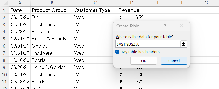
I recommend that each data set in each of the worksheets is housed in an Excel table. You can easily do this by selecting a single cell in the data set and then use the shortcut key CTRL T to create the table. You will then need to click OK to confirm.

You should also give each table a name and you can do that on Excel’s Ribbon: make sure the Table Design tab is selected and then on the far left of the Ribbon enter a name in the Table Name box.

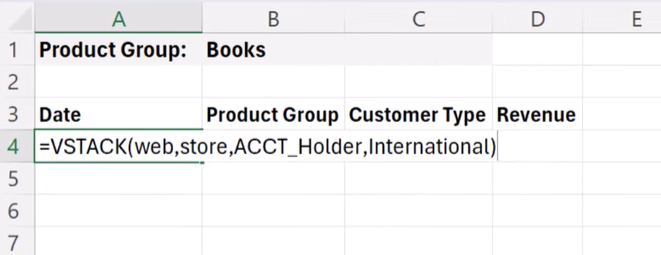
So in my new worksheet where I am going to perform the filter, I first use the VSTACK function to stack the data together. As you can see below I list the tables separated with a comma: =VSTACK(web,store,ACCT_Holder,International)

I then use the FILTER function where VSTACK provides the array. The includes argument also needs to use VSTACK, but this time I specify which column within each table I am applying the criteria to. The column in my example is the Product Group column. Notice the square brackets used to specify the column. =FILTER(VSTACK(web,store,ACCT_Holder,International),VSTACK(web[Product Group],VSTACK(store[Product Group]),VSTACK(ACCT_Holder[Product Group]),VSTACK(International[Product Group])=B1)

Use ENTER on your keyboard to confirm and return the filtered results.

Great article. I’m facing some of these issues as well..
What’s up, I desire to subscribe for this weblog to take most up-to-date updates, so where can i do it please assist.
Wonderful, what a weblog it is! This blog presents useful data to us, keep it up.
Hello to every body, it’s my first pay a visit of this webpage;
this web site carries awesome and really fine stuff in favor of visitors.
Hello, i believe that i saw you visited my site thus
i came to go back the choose?.I’m trying to find things to
improve my web site!I suppose its good enough to use a few of your
ideas!!
Nice post. I was checking continuously this blog and I’m impressed!
Extremely useful information specially the last part :
) I care for such information much. I was looking for this certain information for a
long time. Thank you and best of luck.
You actually make it seem so easy with your presentation but I find this topic to be really
something which I think I would never understand. It seems too complex and
very broad for me. I am looking forward for
your next post, I’ll try to get the hang of it!